10.2. Getting Started - Basic MPC Regulation State Feedback Example

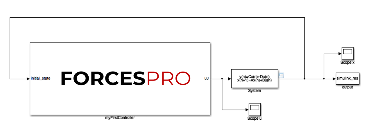
This example will show how to get started with the Simulink® interface of FORCESPRO by designing an MPC regulator for the system below.

You can download the Matlab code of this example to try it out for yourself by clicking here.

\[ \begin{align}\begin{aligned}\begin{split}x_{k+1} = \begin{pmatrix} 0.7115 & −0.4345 \\ 0.4345 & 0.8853 \end{pmatrix}&x_k+ \begin{pmatrix} 0.2173 \\ 0.0573 \end{pmatrix}u_k \\\end{split}\\y_k = \begin{pmatrix} 0 & 1 \end{pmatrix} &x_k\end{aligned}\end{align} \]

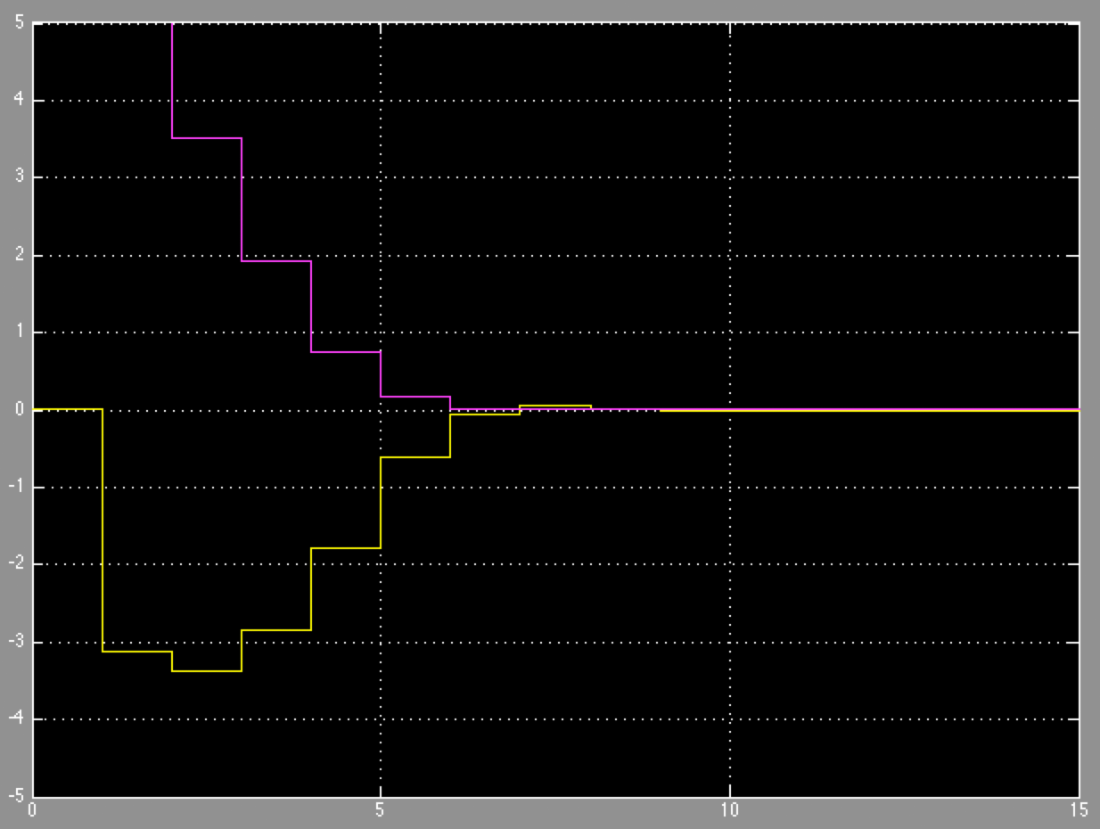
In addition to the task of steering the two states to zero, there are constraints on the single actuator \(u\) and on the second state \(x_2\). We require that the actuator \(u\) does not exceed \([−5,5]\) and the state \(x_2 \geq 0\) for all time. After downloading the files we can start with the design of the controller. First load the data from myFirstController_data.mat into the workspace and then open the Simulink® model myFirstController_sim.slx.

Then copy the FORCESPRO Simulink® block MPC_lib_2012b.mdl into your Simulink® diagram. Give the block a name. Here we will call it myFirstController.

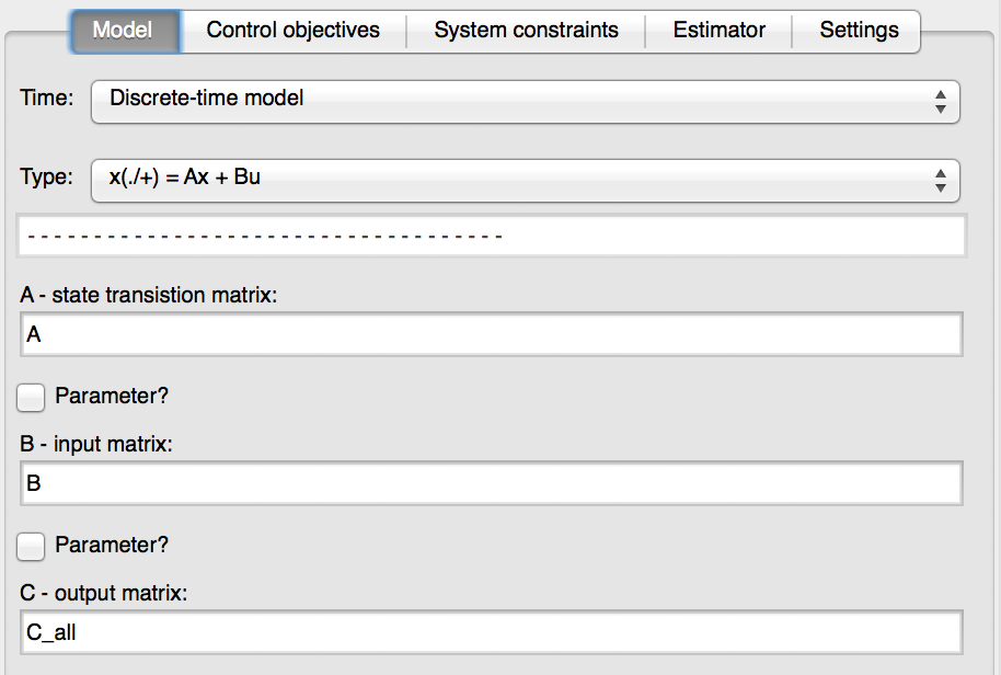
We are now ready to configure the controller. Double-click on the block and go to the ‘Model’ tab to enter the details of the system that we want to control. The model described above has already been discretized with a sampling time of \(0.1\) seconds. We therefore choose ‘Discrete-time model’ and chose the type of state-space model (we have no additive term \(g\) in this example). Enter the state transition matrix \(A\), the input matrix \(B\) and the output matrix \(C_{all}\). Notice that we use \(C_{all}\), which is just the identity matrix, instead of \(C\), since we want to regulate both states, not just the output of the system.

We are now ready to configure the controller. Double-click on the block and go to the ‘Model’ tab to enter the details of the system that we want to control. The model described above has already been discretized with a sampling time of \(0.1\) seconds. We therefore choose ‘Discrete-time model’ and chose the type of state-space model (we have no additive term \(g\) in this example). Enter the state transition matrix \(A\), the input matrix \(B\) and the output matrix \(C_{All}\). Notice that we use \(C_{All}\), which is just the identity matrix, instead of \(C\), since we want to regulate both states, not just the output of the system.

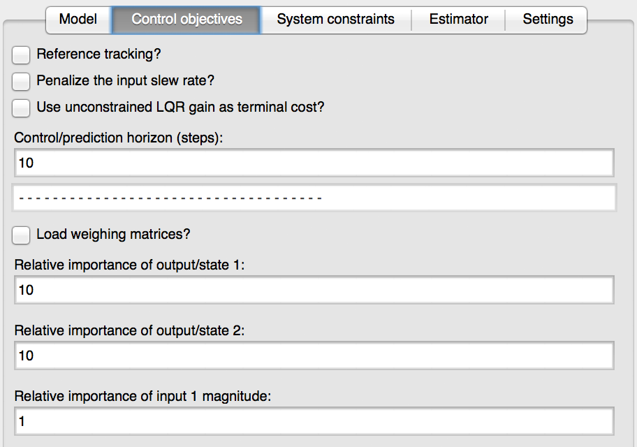
In the ‘Control Objective’ tab we choose a prediction horizon of \(10\) steps, i. e. the controller looks \(1\) second into the future. We will input the relative weights manually. We weight the importance of regulating the states \(10\) times higher then reducing the use of the actuator.

You are encouraged to change these weights and observe the effect on the control behaviour.

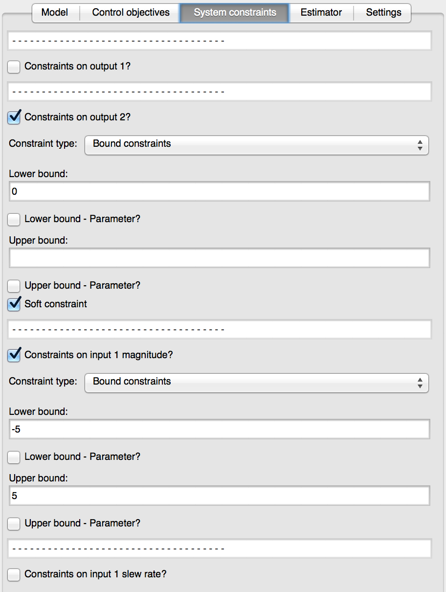
In the ‘System Constraints’ tab we input the details of the constraints described above. The second state must remain positive, whereas the first state is left unconstrained. We also have a constraint on the actuator. We enter the lower bound \(−5\) and the upper bound \(5\). We can also check the option ‘Soft Constraint’ for the output constraint to prevent infeasibility problems in the solver.

Since we are designing a state feedback controller we will leave the only option in the ‘Estimator’ tab as ‘State Feedback’. There will be no estimator built into the FORCESPRO block.

If we wish the controller to give information on the optimization process at each time step we check the option ‘Get Solve Information’ in the ‘Settings’ tab. The controller will have an additional output from which we can read this information.

We are now ready to configure the controller. Simply type

>> configure_block

in the MATLAB® command prompt. This will send a request to the server which will generate a custom controller for your problem. The code is downloaded to your machine and the FORCESPRO block is automatically updated and made ready for simulation on your Simulink® diagram. We can connect the ports of the controller to the rest of the system and run the simulation.

From the left plot we can see that the actuator remains in the allowed range. The right plot shows how the second state \(x_2\) is always non-negative (purple graph in the right plot) and both states are regulated to zero.